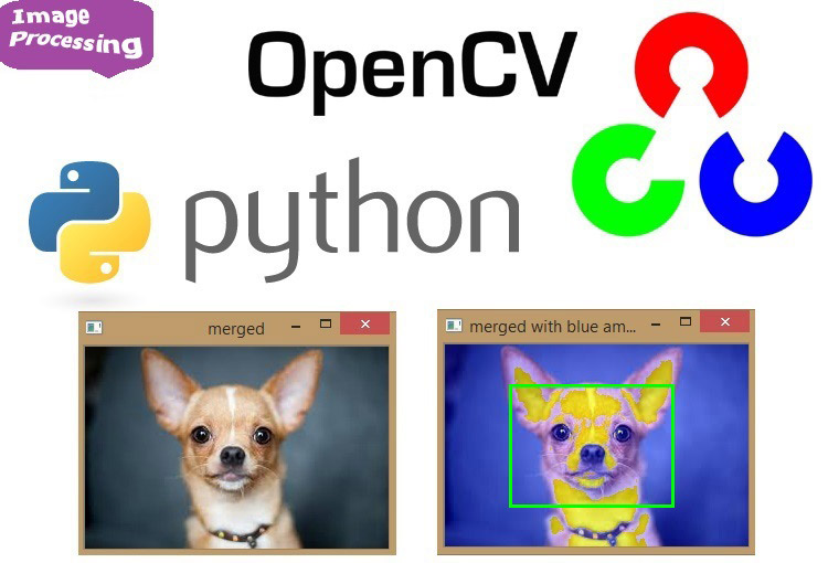
Art is a way of seeing, and they say seeing is believing, but the opposite is also true, believing is seeing and it’s really hard to imagine living in this world without the gift of vision – our eyes, how wonderful it is being an infant when our eyes just open we see the world and started to recognize and see the world around us but as the time passes by, the same wonderful experience becomes a mundane one. But as we are progressing with the technology we are at a verge where the machines are also able to see and understand it. Currently, it doesn’t seem to be a sci-fi if you just unlock your phone with your face, but the story of the development of the machine vision is dated long back to more than 20 years.
The initial formal step in this field was taken back in 1999 in an Intel initiative, when all the research going on was collaborated under the OPEN CV (Open Source computer vision), originally written in C++, with its first major release 1.0 in 2006 second in 2009, third in 2015 and fourth just now in 2018. Now OpenCV has C++, Python and Java interfaces and supports Windows, Linux, Mac OS, iOS and Android. So it can be easily installed in Raspberry Pi with Python and Linux environment. And Raspberry Pi with OpenCV and attached camera can be used to create many real time image processing applications like Face detection, face lock, object tracking, car number plate detection, Home security system etc.
Before going into to learn image processing using openCV it’s important to know what images are and how humans and machines perceive those images.
What are Images?
Images are a two-dimensional representation of the visible light spectrum. And the visible light spectrum is just a part of the electromagnetic spectrum lying there between infrared and ultraviolet spectrum.
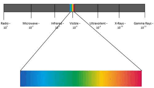
How are images formed: - when a light reflects off an object onto a film, a sensor or on retina.
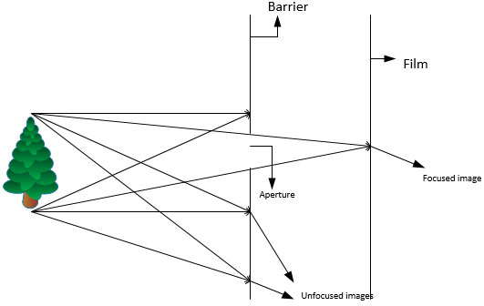
This is how our eyes work, using a barrier to block the most point of lights leaving a small opening through which light can pass it is called as aperture, and it forms a much focused image and is a working model for a pin hole camera, but there is a problem in a pin hole camera, that same amount of light will be entering the aperture, which could not be suitable for the film or image formed also we can’t get a focused image, so as to focus the image we need to move film back and forth, but this is problematic in many situations.
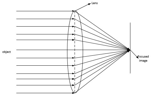
Or we can fix this problem by using lenses, it allows us to control the aperture size, and in photography its known as fStop, generally lower the value of fStop is better in photography.
Aperture size also let us get into nice depth of field called as Bokeh in photography, it allows us to have a blurred background while we focus on image.
How computer stores images
You may have heard of various image formats like .PNG, .JPEG and etc. all of this are digital representation of our analog world, computers do it by translating the image into digital code for storage and then interpret the file back into an image for display. But at the basics they use a common platform for storing the images, and same is true for the openCV.
OpenCV uses RGB (red, green and blue) color space by default for its images, where each pixel coordinate (x, y) contains 3 values ranging for intensities in 8-bit form i.e. (0-255, 28).
Mixing different intensities of each color gives us the full spectrum, that’s why in painting or art these three colors are regarded as primary colors and all others as secondary, because most of the secondary colors can be formed by primary colors. Like for yellow, we have the following values: Red – 255; Green – 255; Blue – 0.
Now the images are stored in multi-dimensional arrays. In programming, array is a series of collection of objects. And here we deal with three type of arrays 1D, 2D and 3D where ‘D’ stands for dimensional.
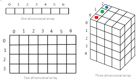
Colored images are stored in three dimensional arrays, where the third dimensions represents the RGB colors (which we will see later), and in together they form different intensities of pixels for an image, while the black & white images are stored in two dimensional arrays and also there are two types of black & white images Greyscale and binary images.
Greyscale images are form from the shades of grey of a two dimensional array [(0,255), (0,255)], while the binary images are of pixels either of black or white.
Why it is difficult for a machine to identify images
Computer vision is a challenging task in itself, you can yourself imagine how hard it is to give a machine a sense of vision, recognition and identification. The following factors are there that makes computer vision so hard.
- Camera sensor and lens limitations
- View point variations
- Changing lighting
- Scaling
- Occlusions
- Object class variations
- Ambiguous Images/Optical Illusions
Application and uses of OpenCV
Despite the difficulty, Computer Vision has many success stories
- Robotic Navigation – Self Driving Cars
- Face Detection & Recognition
- Search Engine Image Search
- License Plate Reading
- Handwriting Recognition
- Snapchat & Face Filters
- Object Recognition
- Ball & Player Tracking in Sports
- And many more!
Installing OpenCV with Python and Anaconda
OpenCV is written in C++, but it’s very much hard to implement it with C++ and hence we choose to implement it with a high level language as python, and also there are additional benefits of implementing OpenCV with python as Python is one of the easiest languages for beginners also It is extremely powerful for data science and machine learning applications and also it stores images in numpy arrays which allows us to do some very powerful operations quite easily.
Basic programming is useful with Exposure to High School Level Math, a webcam, Python 2.7 or 3.6 (Anaconda Package is preferred).
Step 1. Download & Install Anaconda Python Package
Go to: https://www.anaconda.com/download and choose according to your machine weather its windows, Linux or mac and you can choose for python 2.7 or python 3.7 version for either 64 Bit systems or 32 Bit systems, but now a days most of the system are 64 bit.
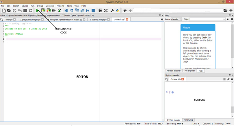
Anaconda distribution of python comes along with Spyder studio, jupyter notebooks and anaconda prompt, which makes python super friendly to use. We would be using spyder studio for doing the examples.
The choice between python 2.7 or 3.7 is completely neutral, but however for the examples we would be using python 3.7 since it’s the future of the python and will take over python 2.7 form 2020, also most of the libraries are being developed in python 3.7 keeping the future aspect of python in mind. Also it also gives the expected results on basic mathematical operations such as (2/5=2.5), while the python 2.7 would evaluate it to 2. Also print is treated as a function in python 3.7 (print(“hello”)), so it gives hands-on to the programmers.
Step 2. Creating a virtual platform with OpenCV
We are going to install OpenCV by creating a virtual platform for spyder by using Anaconda prompt and the YML file uploaded here.
With the YML files we will install all the packages and libraries that would be needed, but however if you want to install any additional packages you can easily install through anaconda prompt, by running the command of that package.
Go to your windows search icon and find anaconda prompt terminal, you can find it inside your anaconda folder that you have just installed.
Then you have to find your downloaded YML file, and from here you have two choices either changing the directory of your terminal to the location where the your YML file is downloaded or either copy your YML file to the directory where your anaconda is installed in most cases it would be inside C:\ drive, after copying your YML file to the specified location RUN the following command on your prompt
conda env create –f virtual_platform_windows.yml
Since my system is running on windows the YML file and the command corresponds to the windows, however you can modify according to your system by replacing windows by linux or mac as respective.
Note: - If the package extraction gives error do install pytorch and numpy first and then run the above command.
Now find the anaconda navigator and there would be a drop down menu of “Applications on ___” and from there select virtual environment and then from there you have to launch Spyder studio.
And that’s it, you’re ready to get started!
Opening and Saving images in OpenCV
Here we are explaining some basic commands and terminology to use Python in OpenCV. We will learn about three basic functions in OpenCV imread, imshow and imwrite.
#comments in python are given by # symbol
Import opencv in python by command
import cv2
Load an image using ‘imread’ specifying the path to the image
image =cv2.imread('input.jpg')
Now that image is loaded and stored in python as a variable we named as image
Now to display our image variable, we use ‘imshow’ and the first parameter for imshow function is the title shown on the image window, and it has to be entered in (‘ ’) to represent the name as a string
cv2.imshow('hello world',image)
waitkey allows us to input information when image window is open, by leaving it blank it just waits for anykey to be pressed before continuing, by placing numbers (except 0), we can specify a delay for how long you keep the window open (time in milliseconds here).
cv2.waitKey()
‘destroyAllWindows’ closes all the open windows, failure to place this will cause your programme to hang.
cv2.destroyAllWindows()

Now let’s take a look how images are stored in open cv, for this we will use numpy, numpy is a library for python programming for adding support to large multidimensional arrays and matrices.
import cv2
#importing numpy
import numpy as np
image=cv2.imread('input.jpg')
cv2.imshow('hello_world', image)
#shape function is very much useful when we are looking at a dimensions of an array, it returns a tuple which gives a dimension of an image
print(image.shape)
cv2.waitKey()
cv2.destroyAllWindows()
console output - (183, 275, 3), The two dimensions of the image are 183 pixels in height and 275 pixels in width and 3 means that there are three other components (R, G, B) that makes this image (it shows that the colored images are stored in three dimensional arrays).
Now let’s print each dimension of image by adding the following lines of code
print('Height of image:',(image.shape[0],'pixels'))
print('Width of image:',(image.shape[1],'pixels'))
console output - Height of image: (183, 'pixels')
Width of image: (275, 'pixels')
Saving the edited image in OpenCV
We use ‘imwrite’ for specifying the filename and the image to be saved.
cv2.imwrite('output.jpg',image)
cv2.imwrite('output.png',image)
First argument is name of the file we want to save, {to read or to save the file we use (‘ ’) to indicate it as a string} and second argument is the file name.
OpenCV allows you to save the image in different formats.
Grey Scaling Image in OpenCV
Greyscaling is the process by which an image is converted from a full color to shades of grey (black and white)
In opencv, many functions greyscales the images before processing. This is done because it simplifies the image, acting almost as a noise reduction and increasing the processing time as there is less information in image (as greyscale images are stored in two dimensional arrays).
import cv2
# load our input image
image=cv2.imread('input.jpg')
cv2.imshow('original', image)
cv2.waitKey()
#we use cvtcolor, to convert to greyscale
gray_image = cv2.cvtColor(image, cv2.COLOR_BGR2GRAY)
cv2.imshow('grayscale', gray_image)
cv2.waitKey()
cv2.destroyALLWindows()
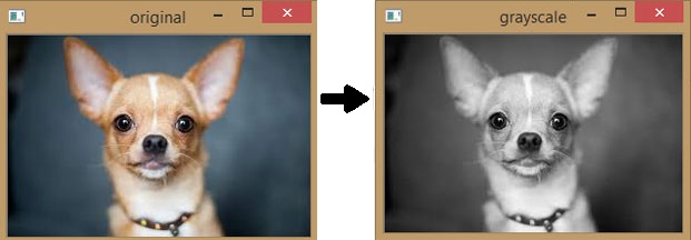
Simpler way to convert image into grayscale is just add the argument 0 in imread function aside to the image name
import cv2
grey_image=cv2.imread('input.jpg',0)
cv2.imshow('grayscale',grey_image)
cv2.waitKey()
cv2.destroyAllWindows()
Now let’s see the dimension of each image by the shape function
import cv2
import numpy as np
image=cv2.imread('input.jpg')
print(image.shape)
cv2.imshow('original', image)
cv2.waitKey()
gray_image = cv2.cvtColor(image, cv2.COLOR_BGR2GRAY)
cv2.imshow('grayscale', gray_image)
print(gray_image.shape)
cv2.waitKey()
cv2.destroyALLWindows()
Console output: - (183, 275, 3) – for colored image
(183, 275) – for grayscale image
Hence it clearly shows that the colored images are represented by three dimensional arrays, while the gray scale images by two dimensional arrays.
Color Spaces
Color spaces are the way the images are stored. RGB, HSV, CMYK are the different color spaces, these are just simple ways to represent color.
RGB – Red, Green and Blue.
HSV – Hue, Saturation and Value.
And CMYK is commonly used in inkjet printers.
RGB or BGR color space
OpenCV’s default color space is RGB. RGB is an additive color model that generates colors by combining blue, green and red colors of different intensities/ brightness. In OpenCV we use 8 bit color depths.
- Red (0-255)
- Blue (0-255)
- Green (0-255)
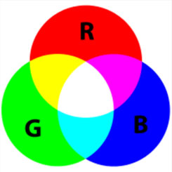
However OpenCV actually stores color in BGR format.
Fun Fact: - We use BGR order in computers due to how unsigned 32-bit integers are stored in memory, it still ends up being stored as RGB. The integer representing a color eg:- 0X00BBGGRR will be stored as 0XRRGGBB.
HSV (Hue, Saturation & value/ Brightness) is a color space that attempts to represent colors the humans perceive it. It stores color information in a cylindrical representation of RGB color points.
Hue – color value (0-179)
Saturation – Vibrancy of color (0-255)
Value – Brightness or intensity (0-255)
HSV color space format is useful in color segmentation. In RGB, filtering specific color isn’t easy, however HSV makes it much easier to set color ranges to filter specific color as we perceive them.
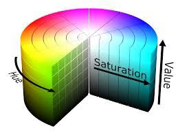
Hue represents the color in HSV, the hue value ranges from 0 – 180 and not 360 so it is not completing the full circle and so it is mapped differently than the standard.

Color range filters
- Red – (165-15)
- Green – (45-75)
- Blue – (90-120)
As we know the images being stored in RGB (Red, Green and Blue) color space and so OpenCV shows us the same, but the first thing to remember about opencv’s RGB format is that it’s actually BGR and we can know it by looking at the image shape.
import cv2
import numpy as np
image = cv2.imread('input.jpg')
#B,G,R value for the first 0,0 pixel
B,G,R=image[0,0]
print(B,G,R)
print(image.shape)
#now if we apply this on grayscale image
gray_img=cv2.cvtColor(image,cv2.COLOR_BGR2GRAY)
print(gray_img.shape)
#gray_image pixel value for 10,50 pixel
print(gray_img[10,50])
Console Output: print(B,G,R) - 6 11 10
print(image.shape) - (183, 275, 3)
print(gray_img.shape) - (183, 275)
print(gray_img[10,50]) - 69
Now there are only two dimensions in a gray scale image, since we remember the color image is stored in three dimensions, the third dimension being the (R,G,B) while in grayscale only two dimensions are present, since (R,G,B) is absent and for a particular pixel position we only get a single value while in colored image we got three values.
Another useful color space is HSV
import cv2
image=cv2.imread('input.jpg')
hsv_image=cv2.cvtColor(image,cv2.COLOR_BGR2HSV)
cv2.imshow('HSV image',hsv_image)
cv2.imshow('Hue channel',hsv_image[:,:,0])
cv2.imshow('saturation channel',hsv_image[:,:,1])
cv2.imshow('value channel',hsv_image[:,:,2])
cv2.waitKey()
cv2.destroyAllWindows()
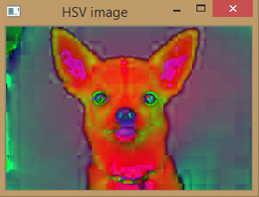
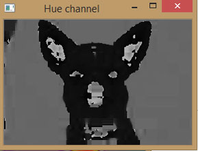
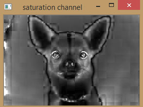

After running the code you can see the four images of which three are of the individual channels and one is combined HSV image.
Hue channel image is quite dark because its value only varies from 0 to 180.
Also, note that imshow function tries to show you the RGB or BGR image, but HSV conversion overlaps it.
Also, the value channel will be similar to the grayscale of image due to its brightness.
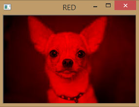
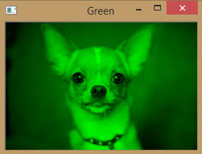
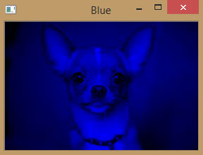
Exploring individual components of RGB image
import cv2
image=cv2.imread('input.jpg')
#opencv's split function splits the imageinti each color index
B,G,R=cv2.split(image)
cv2.imshow("Red",R)
cv2.imshow("Green",G)
cv2.imshow("Blue",B)
#making the original image by merging the individual color components
merged=cv2.merge([B,G,R])
cv2.imshow("merged",merged)
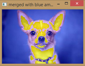
#amplifying the blue color
merged=cv2.merge([B+100,G,R])
cv2.imshow("merged with blue amplify",merged)
#representing the shape of individual color components.
# the output wuld be only two dimension whih wouldbe height and width, since third element of RGB component is individually represented
print(B.shape)
print(R.shape)
print(G.shape)
cv2.waitKey(0)
cv2.destroyAllWindows()
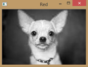
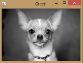
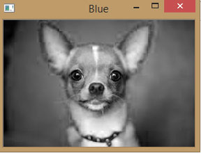
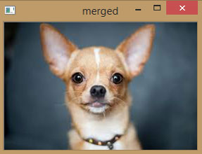
Console output: #dimensions of image from shape function
(183, 275)
(183, 275)
(183, 275)
Converting image into individual RGB component
In below code we have created a matrix of zeros with the dimensions of image HxW, zero return an array filled with zeros but with same dimensions.
Shape function is very much useful when we are looking at the dimension of an image, and here we have done slicing of that shape function. So shape[:2] would grab everything up to designated points i.e. upto second designated points which would be height and width of the image as third represents RGB component of image and we don't need it here.
import cv2
import numpy as np
image = cv2.imread('input.jpg')
B,G,R = cv2.split(image)
zeros=np.zeros(image.shape[:2],dtype="uint8")
cv2.imshow("RED",cv2.merge([zeros,zeros,R]))
cv2.imshow("Green",cv2.merge([zeros,G,zeros]))
cv2.imshow("Blue",cv2.merge([B,zeros,zeros]))
cv2.waitKey(0)
cv2.destroyAllWindows()
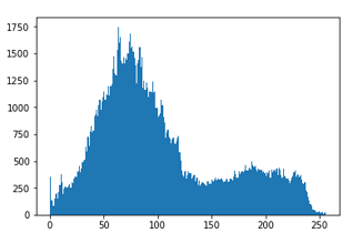
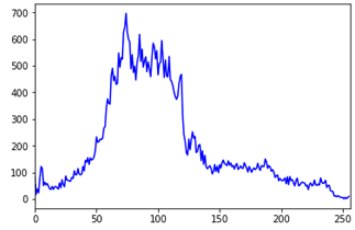
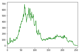
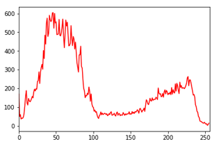
Histogram Representation of Image
Histogram representation of image is the method of visualizing the components of images.
The following code lets you analyze the image through the color histogram of its combined and individual color components.
import cv2
import numpy as np
#we need to import matplotlib to create histogram plots
import matplotlib.pyplot as plt
image=cv2.imread('input.jpg')
histogram=cv2.calcHist([image],[0],None,[256],[0,256])
#we plot a histogram, ravel() flatens our image array
plt.hist(image.ravel(),256,[0,256])
plt.show()
#viewing seperate color channels
color=('b','g','r')
#we know seperate the color and plot each in histogram
for i, col in enumerate (color):
    histogram2=cv2.calcHist([image],[i],None,[256],[0,256])
    plt.plot(histogram2,color=col)
    plt.xlim([0,256])
    plt.show()
Let’s understand the calcHist function with each of its individual parameters
cv2.calcHist(images, channels, mask, histsize, ranges)
Images: its the source image of type uint 8 or float 32. It should be given in square brackets, i.e. “[img]”, which also indicate its second level array since an image for opencv is data in an array form.
Channels: it is also given in square brackets. It is the index of channel for which we calulate histogram, for example if input is grayscale image its value is [0], for color images you can pass [0], [1] or [2] to calculate histogram of blue, green and red channel respectively.
Mask: mask image. to find the histogram of full image, it is given as “none”. but if you want to find the histogram of particular region of image, you have to create a mask image for that and give it as a mask.
Histsize: This represents our BIN count. Needed to be given in square brackets for full scale we pass [256].
Ranges: This is our range, normally is [0,256]
Drawing Images and Shapes using OpenCV
Below are few Examples for drawing lines, rectangle, polygon, circle etc in OpenCV.
import cv2
import numpy as np
#creating a black square
image=np.zeros((512,512,3),np.uint8)
#we can also create this in black and white, however there would not be any changes
image_bw=np.zeros((512,512),np.uint8)
cv2.imshow("black rectangle(color)",image)
cv2.imshow("black rectangle(B&W)",image_bw)
Line
#create a line over black square
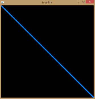
#cv2.line(image, starting coordinates, ending coordinates, color, thickness)
#drawing a diagonal line of thickness 5 pixels
image=np.zeros((512,512,3),np.uint8)
cv2.line(image,(0,0),(511,511),(255,127,0),5)
cv2.imshow("blue line",image)
Rectangle
#create a rectangle over a black square
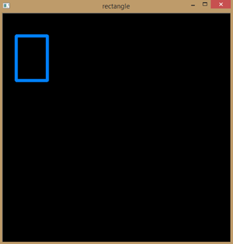
#cv2.rectangle(image,starting coordinates, ending coordinates, color, thickness)
#drawing a rectangle of thickness 5 pixels
image=np.zeros((512,512,3),np.uint8)
cv2.rectangle(image,(30,50),(100,150),(255,127,0),5)
cv2.imshow("rectangle",image)
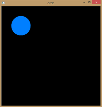
#creating a circle over a black square
#cv2.circle(image,center,radius,color,fill)
image=np.zeros((512,512,3),np.uint8)
cv2.circle(image,(100,100),(50),(255,127,0),-1)
cv2.imshow("circle",image)
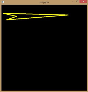
#creating a polygon
image=np.zeros((512,512,3),np.uint8)
#lets define four points
pts=np.array([[10,50], [400,60], [30,89], [90,68]], np.int32)
#lets now reshape our points in form required by polylines
pts=pts.reshape((-1,1,2))
cv2.polylines(image, [pts], True, (0,255,255), 3)
cv2.imshow("polygon",image)
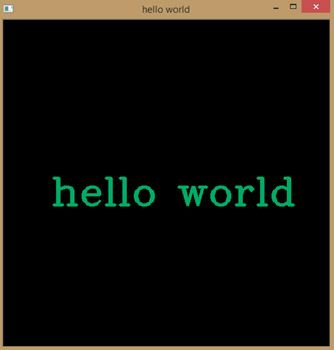
#putting text using opencv
#cv2.putText(image,'text to display',bootom left starting point, font,font size, color, thickness)
image=np.zeros((512,512,3),np.uint8)
cv2.putText(image,"hello world", (75,290), cv2.FONT_HERSHEY_COMPLEX,2,(100,170,0),3)
cv2.imshow("hello world",image)
cv2.waitKey(0)
cv2.destroyAllWindows()
Computer Vision and OpenCV are very vast topics to cover but this guide would be good starting point to learn OpenCV and image processing.


